Chapter 14. Runtime Optimization

ABSTRACT Runtime optimization has become an important technique for the implementation of many programming languages. The move from ahead-of-time compilation to runtime optimization lets the language runtime and its compilers capitalize on facts that are not known until runtime. If these facts enable specialization of the code, such as folding an invariant value, avoiding type conversion code, or replacing a virtual function call with a direct call, then the profit from use of runtime information can be substantial.

This chapter explores the major issues that arise in the design and implementation of a runtime optimizer. It describes the workings of a hot-trace optimizer and a method-level optimizer; both are inspired by successful real systems. The chapter lays out some of the tradeoffs that arise in the design and implementation of these systems.

KEYWORDS Runtime Compilation, Just-in-Time Compilation, Dynamic Optimization

14.1 Introduction

Runtime optimization code optimization applied at runtime

Many programming languages include features that make it difficult to produce high-quality code at compile time. These features include late binding, dynamic loading of both declarations and code (classes in JAVA), and various kinds of polymorphism. A classic compiler, sometimes called an ahead-of-time compiler (AOT), can generate code for these features. In many cases, however, it does not have sufficient knowledge to optimize the code well. Thus, the AOT compiler must emit the generic code that will work in any situation, rather than the tailored code that it might generate with more precise information.

For some problems, the necessary information might be available at link time, or at class-load time in JAVA. For others, the information may not be known until runtime. In a language where such late-breaking information can have a significant performance impact, the system can defer optimization or translation until it has enough knowledge to produce efficient code.

Compiler writers have applied this strategy, runtime optimization or just-in-time compilation (JIT), in a variety of contexts, ranging from early LISP systems through modern scripting languages. It has been used to build regular-expression search facilities and fast instruction-set emulators. This chapter describes the technical challenges that arise in runtime optimization and runtime translation, and shows how successful systems have addressed some of those problems.

Just-in-time compilers are, undoubtedly, the most heavily used compilers that the computer science community has built. Most web browsers include JITs for the scripting languages used in web sites. Runtime systems for languages such as JAVA routinely include a JIT that compiles the heavily used code. Because these systems compile the code every time it runs, they perform many more compilations than a traditional AOT compiler.

Conceptual Roadmap

Classic AOT compilers make all of their decisions based on the facts that they can derive from the source text of the program. Such compilers can generate highly efficient code for imperative languages with declarations. However, some languages include features that make it impossible for the compiler to know important facts until runtime. Such features include dynamic typing, some kinds of polymorphism, and an open class structure.

Runtime optimization involves a fundamental tradeoff between time spent compiling and code quality. The runtime optimizer examines the program's state to derive more precise information; it then uses that knowledge to specialize the executable code. Thus, to be effective, the runtime optimizer must derive useful information. It must improve runtime performance enough to compensate for the added costs of optimization and code generation. The compiler writer, therefore, has a strong incentive to use methods that are efficient, effective, and broadly applicable.

A Few Words About Time

Runtime optimization adds a new layer of complexity to our reasoning about time. These techniques intermix compile time with runtime and incur compile-time costs every time a program executes.

JIT time We refer to the time when the runtime opti- mizer or the just-in-time compiler is, itself, executing as JIT time.

At a conceptual level, the distinction between compile time and runtime remains. The runtime optimizer plans runtime behavior and runtime data structures, just as an AOT compiler would. It emits code to create and maintain the runtime environment. Thus, JIT-time activities are distinct from runtime activities. All of the reasoning about time from earlier chapters is relevant, even if the time frame when the activities occur has shifted.

To further complicate matters, some systems that use runtime optimization rely on an interpreter for their default execution mode. These systems interpret code until they discover a segment of code that should be compiled. At that point they compile and optimize the code; they then arrange for subsequent executions to use the compiled code for the segment. Such systems intermix interpretation, JIT compilation, and execution of compiled code.

Overview

To implement efficiently features such as late binding of names to types or classes, dynamic loading and linking of code, and polymorphism, compiler writers have turned to runtime optimization. A runtime optimizer can inspect the running program's state to discover information that was obscured or unavailable before runtime.

Runtime compilation also provides nat- ural mechanisms to deal with runtime changes in the program’s source text (see Section 14.5.4).

By runtime, the system mostly knows what code is included in the executable. Late bound names have been resolved. Data structures have been allocated, so their sizes are known. Objects have been instantiated, with full class information. Using facts from the program's runtime state, a compiler can specialize the code in ways that are not available to an AOT compiler.

Runtime compilation has a long history. McCarthy's early LISP systems compiled native code for new functions at runtime. Thompson's construction, which builds an NFA from a regular expression, was invented to compile an RE into native code inside the search command for the QED editor--one of the first well-known examples of a compiler that executed at runtime. Subsequent systems used these techniques for purposes that ranged from the implementation of dynamic object-oriented languages such as SMALLtalk-80 through code emulation for portability. The rise of the World Wide Web was, in part, predicated on widespread use of JAVA and JAVASCRIPT, both of which rely on runtime compilation for efficiency.

Runtime optimization presents the compiler writer with a novel set of challenges and opportunities. Time spent in the compiler increases the overall running time, so the JIT writer must balance JIT costs against expected improvement. Techniques that shift compilation away from infrequently executed, or cold, code and toward frequently executed, or hot, code can magnify any gain from optimization.

We use the term JIT to cover all runtime optimizers, whether their input is source code, as in McCarthy's early LISP systems; some high-level notation, as in Thompson's RE-to-native-code compiler; some intermediate form as in JAVA systems; or even native code, as in Dynamo. The digressions throughout this chapter will introduce some of these systems, to familiarize the reader with the long history and varied applications of these ideas.

Impact of JIT Compilation

The data was gathered on OpenJDK version 1.8.0_292 running on an Intel ES2640 at 2.4GHz.

The input codes had uniform register pres- sure of 20 values. The allocator was allotted 15 registers.

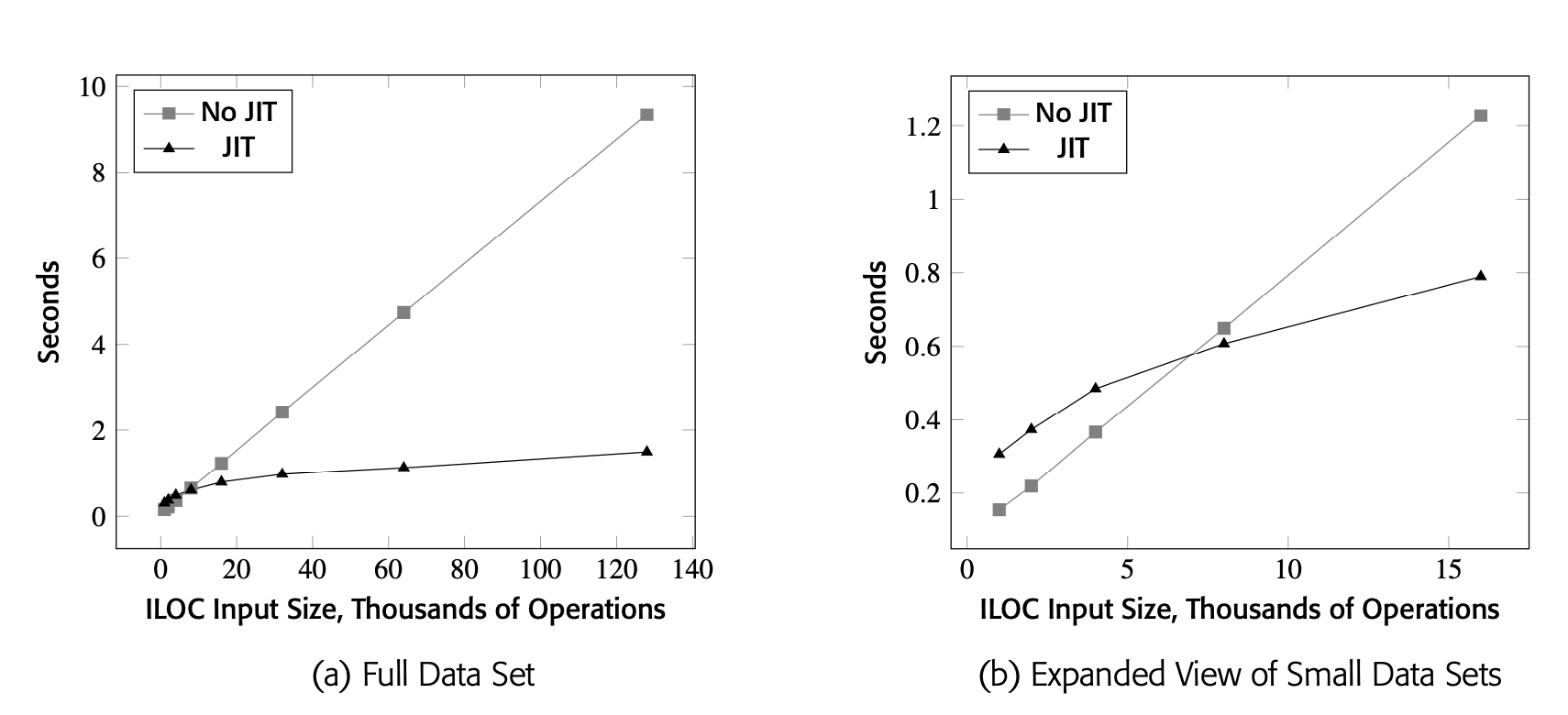
JIT compilation can make a significant difference in the execution speed of an application. As a concrete example, Fig. 14 shows the running times of a JAVA implementation of the local register allocation algorithm from Section 13.3. Panel (a) shows the running time of the allocator on a series of blocks with 1,000 lines, 2,000 lines, 4,000 lines, and so on up to 128,000 lines of ILOC code. The gray line with square data points shows the running time with the JIT disabled; the black line with triangular data points shows the running time with the JIT enabled. Panel (b) zooms in on the startup behavior--that is, the smaller data sets.

These numbers are specific to this single application. Your experience will vary.

The JIT makes a factor of six difference on the largest data set; it more than compensates for the time spent in the JIT. Panel (a) shows the JIT's contribution to the code's performance. Panel (b) shows that VM-code emulation is actually faster on small data sets. Time spent in the JIT slows execution in the early stages of runtime; after roughly one-half second, the speed advantage of the compiled code outweighs the costs incurred by the JIT.

Roadmap

JIT design involves fundamental tradeoffs between the amount of work performed ahead of time, the amount of work performed in the JIT, and the improvement that JIT compilation achieves. As languages, architectures, and runtime techniques have changed, these tradeoffs have shifted. These tradeoffs will continue to shift and evolve as the community's experience with building and deploying JITs grows. Our techniques and our understanding will almost certainly improve, but the fundamental tradeoff of efficiency against effectiveness will remain.

This chapter provides a snapshot of the state of the field at the time of publication. Section 14.2 describes four major issues that play important roles in shaping the structure of a JIT-enabled system. The next two sections present high-level sketches for two JITs that sit at different points in the design space. Section 14.3 describes a hot-trace optimizer while Section 14.4 describes a hot-method optimizer; both designs are modeled after successful systems. The Advanced Topics section explores several other issues that arise in the design and construction of practical JIT-based systems.

14.2 Background

Runtime optimization has emerged as a technology that lets the runtime system adapt the executable code more closely to the context in which it executes. In particular, by deferring optimization until the compiler has more complete knowledge about types, constant values, and runtime behavior (e.g., profile information), a JIT compiler can eliminate some of the overhead introduced by language features such as object-orientation, dynamic typing, and late binding.

Success in runtime optimization, however, requires attention to both the efficiency and the effectiveness of the JIT. The fundamental principle of runtime optimization is

$A runtime compiler must save more cycles than it uses.$

If the runtime compiler fails to meet this constraint, then it actually slows down the application's execution.

This critical constraint shapes both the JIT and the runtime system with which it interacts. It places a premium on efficiency in the compiler itself. Because compile time now adds to running time, the JIT implementation's efficiency directly affects the application's running time. Both the scope and ambition of the JIT matter; both asymptotic complexity and actual runtime overhead matter. Equally important, the scheme that chooses which code segments to optimize has a direct impact on the total cost of running an application.

This constraint also places a premium on the effectiveness of each algorithm that the JIT employs. The compiler writer must focus on techniques that are both widely applicable and routinely profitable. The JIT should apply those techniques to regions where opportunities are likely and where those improvements pay off well. A successful JIT improves the code's running time often enough that the end users view time spent in the JIT as worthwhile.

Regular expression search in the QED editor Ken Thompson built a regular-expression (RE) search facility into the QED editor in the late 1960s. This search command was an early JIT compiler, invoked under the user's direction. When the user entered an RE, the editor invoked the JIT to create native code for the IBM 7094. The editor then invoked the native code to perform the search. After the search, it discarded the code.

The JIT was a compiler. It first parsed the RE to check its syntax. Next, it converted the RE to a postfix notation. Finally, it generated native code to perform the search. The JIT's code generator used the method now known as Thompson's construction to build, implicitly, an NFA (see Section 2.4.2). The generated code simulated that NFA. It used search to avoid introducing duplicate terms that would cause exponential growth in the runtime state.

The QED search command added a powerful capability to a text editor that ran on a 0.35 MIP processor with 32 KB of RAM. This early use of JIT technology created a responsive tool that ran in this extremely constrained environment.

This situation differs from that which occurs in an AOT compiler. Compiler writers assume that the code produced by an AOT compiler executes, on average, many times per compilation. Thus, the cost of optimization is a small concern. AOT compilers apply a variety of transformations that range from broadly applicable methods such as value numbering to highly specific ones such as strength reduction. They employ techniques that produce many small improvements and others that produce a few large improvements. An AOT compiler wins by accumulating the improvements from a suite of optimizations, used at every applicable point in the code. The end user is largely insulated from the cost of compilation and optimization.

To recap, the constraints in a JIT mean that the JIT writer must choose transformations well, implement them carefully, and apply them to regions that execute frequently. Fig. 14.1 demonstrates the improvement from JIT compilation with the HotSpot Server Compiler. In that test, HotSpot produced significant improvements for codes that ran for more than one-half of a second. Careful attention to both costs and benefits allows this JIT to play a critical role in JAVA's runtime performance.

14.2.1 Execution Model

The choice of an $execution model$ has a large impact on the shape of a runtime optimization system. It affects the speed of baseline execution. It affects the amount of compilation that the system must perform and, therefore,the cumulative overhead of optimization. It also affects the complexity of the implementation.

A runtime optimization system can be complex. It takes, as input, code for some virtual machine (VM) code. The VM code might be code for an abstract machine such as the JAVA VM (JVM) or the Smalltalk-80 VM. In other systems, the VM code is native machine code. As output, the runtime optimizer produces the results of program execution.

The difference between these modes is largely transparent to the user.

The runtime system can produce results by executing native code, by interpreting VM code, or by JIT compiling VM code to native code and running it. The relationship between the JIT, the code, and the rest of the runtime system determines the mode of execution. Does the system execute, by default, native code or VM code? Either option has strengths and weaknesses.

native-code execution usually implies JIT compilation before execution, unless the VM code is native code.
VM-code execution usually implies interpretation at some level. The code is compact; it can be more abstract than native code.

Native-code execution is, almost always, faster than VM-code execution. Native code relies on hardware to implement the fetch-decode-execute cycle, while VM emulation implements those functions in software. Lower cost per operation turns into a significant performance advantage for any nontrivial execution.

A VM-code system can defer scanning and parsing a procedure until it is called. The savings in startup time can be substantial.

On the other hand, VM-code systems may have lower startup costs, since the system does not need to compile anything before it starts to execute the application. This leads to faster execution for short-running programs, as shown in Fig. 14.1(b). For procedures that are short or rarely executed, VM-code emulation may cost less than JIT compilation plus native-code execution.

The Deutsch-Schiffman SMALLTALK-80 system used three formats for an AR.

It translated between formats based on whether or not the code accessed the AR as data.

The introduction of a JIT to a VM-code system typically creates a mixed-mode platform that executes both VM code and native code. A mixed-mode system may need to represent critical data structures, such as activation records, in both the format specified for the VM and the format supported by the native ISA. The dual representations may introduce translation between VM-code structures and native-code structures; those translations, in turn, will incur runtime costs.

ADAPTIVE FORTRAN Adaptive Fortran was a runtime optimizer for FORTRAN IV built by Hansen as part of the work for his 1974 dissertation. He used it to explore both the practicality and the profitability of runtime optimization. Adaptive Fortran introduced many ideas that are found in modern systems.

The system used a fast ahead-of-time compiler to produce an IR version of the program; the IR was grouped into basic blocks. At runtime, the IR was interpreted until block execution counts indicated that the block could benefit from optimization. (The AOT compiler produced block-specific, optimization-specific thresholds based on block length, nesting depth, and the cost of the JIT optimization.)

Guided by the execution counts and thresholds, a supervisor invoked a JIT to optimize blocks and their surrounding context. The use of multiple block-specific thresholds led to an effect of progressive optimization—more optimizations were applied to blocks that accounted for a larger share of the running time.

One key optimization, which Hansen called fusion, aggregated together multiple blocks to group loops and loop nests into segments. This strategy allowed Adaptive Fortran to apply loop-based optimizations such as code motion.

The alternative, native-code execution, distributes the costs in a different way. Such a system must compile all vm code to native code, either in an AOT compilation or at runtime. The AOT solution leads to fully general code and, thus, a higher price for nonoptimized native execution. The JIT solution leads to a system that performs more runtime compilation and incurs those costs on each execution.

There is no single best solution to these design questions. Instead, the compiler writer must weigh carefully a variety of tradeoffs and must implement the system with an eye toward both efficiency and effectiveness. Successful systems have been built at several points in this design space.

14.2.2 Compilation Triggers

The runtime system must decide when and where to invoke the JIT. This decision has a strong effect on overall performance because it governs how often the JIT runs and where the JIT focuses its efforts.

Runtime optimizers use JIT compilation in different ways. If the system JIT compiles all code, as happens in some native-code systems, then the trigger may be as simple as "compile each procedure before its first call." If, instead,the system only compiles hot code, the trigger may require procedure-level or block-level profile data. Native-code environments and mixed-mode environments may employ different mechanisms to gather that profile data.

In a native-code environment, the compiler writer must choose between (1) a system that works from VM code and compiles that VM code to native code before it executes, or (2) a system that works from AOT-compiled native code and only invokes the JIT on frequently executed, or hot, code. The two approaches lead to distinctly different challenges.

VM-Code Execution

In a mixed-mode environment, the system can begin execution immediately and gather profile data to determine when to JIT compile code for native execution. These systems tend to trigger compilation based on profile data exceeding a preset threshold value above which the code is considered hot. This approach helps the system avoid spending JIT cycles on code that has little or no impact on performance.

Threshold values play a key role in determining overall runtime. Larger threshold values decrease the number of JIT compilations. At the same time, they increase the fraction of runtime spent in the VM-code emulator, which is typically slower than native-code execution. Varying the threshold values changes system behavior.

Backward branch In this context, a backward branch or jump targets an address smaller than the program counter. Loop-closing branches are usually back- ward branches.

To obtain accurate profile data, a VM-code environment can instrument the application's branches and jumps. To limit the overhead of profile collection, these systems often limit the set of points where they collect data. For example, blocks that are the target of a backward branch are good candidates to profile because they are likely to be loop headers. Similarly, the block that starts a procedure's prolog code is an obvious candidate to profile. The system can obtain call-site specific data by instrumenting precall sequences. All of these metrics, and others, have been used in practical and effective systems.

Native-Code Execution

If the system executes native code, it must compile each procedure before that code can run. The system can trigger compilation at load time, either in batch for the entire executable (Speed Doubler) or as modules are loaded (early versions of the V8 system for JAVASCRIPT). Alternatively, the system can trigger the compiler to translate each procedure the first time it runs. To achieve that effect, the system can link a stub in place of any yet-to-be-compiled procedure; the stub locates the VM code for the callee, JIT compiles and links it, and reexecutes the call.

SPEED DOUBLER Speed Doubler was a commercial product from Connectix in the 1990s. It used load-time compilation to retarget legacy applications to a new ISA. Apple had recently migrated its Macintosh line of computers from the Motorola MC 68000 to the IBM POWER PC. Support for legacy applications was provided by an emulator built into the MacOS.

Speed Doubler was a load-time JIT that translated MC 68000 applications into native POWER PC code. By eliminating the emulation overhead, it provided a substantial speedup. When installed, it was inserted between the OS loader and the start of application execution. It did a quick translation, then branched to the application’s startup code.

The initial version of Speed Doubler appeared to perform an instruction-by- instruction translation, which provided enough improvement to justify the product’s name. Subsequent versions provided better runtime performance; we presume it was the result of better optimization and code generation. Speed Doubler used native-code execution with a compile-on-load discipline to provide a simple and transparent mechanism to improve running times. Users perceived that JIT compilation cost significantly less than the speedups that it achieved, so the product was successful.

Load-time strategies must JIT-compile every procedure, whether or not it ever executes. Any delay from that initial compilation occurs as part of the application’s startup. Compile-on-call shifts the cost of initial compilation later in execution. It avoids compiling code that never runs, but it does com- pile any code that runs, whether it is hot or cold.

Decreasing time in the JIT directly reduces elapsed execution time.

If the system starts from code compiled by an AOT compiler, it can avoid these startup compilations. The AOT compiler can insert the necessary code to gather profile data. It might also annotate the code with information that may help subsequent JIT compilations. A system that uses precompiled na- tive code only needs to trigger the optimizer when it discovers that some code fragment is hot—that is, the code consumes enough runtime to justify the cost of JIT compiling it.

Hot Traces A trace optimizer watches runtime branches and jumps to discover hot traces. Once a trace's execution count exceeds the preset hot threshold, the system invokes the jit to construct an optimized native-code implementation of the trace.

Trace optimizers perform local or regional optimization on the hot trace, followed by native-code generation including allocation and scheduling. Because a runtime trace may include calls and returns, this "regional" optimization can make improvements that would be considered interprocedural in an AOT compiler.

Hot Methods A method optimizer finds procedures that account for a significant fraction of overall running time by monitoring various counters. These counters include call counts embedded in the prolog code, loop iteration counts collected before backward branches, and call-site specific data gathered in precall sequences. Once a method becomes hot, the system uses a jit to compile optimized native code for the method. Because it works on the entire method, the optimizer can perform nonlocal optimizations, such as code motion, regional instruction scheduling, dead-code elimination, global redundancy elimination, or strength reduction. Some method optimizers also perform inline substitution. They might pull inline the code for a frequently executed call in the hot method. If most calls to a hot method come from one call site, the optimizer might inline the callee into that caller.

The choice of granularity has a profound impact on both the cost of optimizations and the opportunities that the optimizer discovers.

Assume a trace that has one entry but might have premature exits.

A trace optimizer might apply lvn to the entire trace to find redundancy, fold constants, and simplify identities. Most method optimizers use a global redundancy algorithm, which is more expensive but should find more opportunities for improvement.

Linear scan achieves some of the benefits of global allocation with lower cost than graph coloring.

A trace optimizer might use a fast local register allocator like the algorithm from Section 13.3. By contrast, a method optimizer must deal with control flow, so it needs a global register allocator such as the coloring allocator or the linear scan allocator (see Sections 13.4 and 13.5.3). Again, the tradeoff comes down to the cost of optimization against the total runtime improvement.

14.2.4 Sources of Improvement

A jit can discover facts that are not known before runtime and use those facts to justify or inform optimization. These facts can include profile information, object types, data structure sizes, loop bounds, constant values or types, and other system-specific facts. To the extent that these facts enable optimization that cannot be done in an AOT compiler, they help to justify runtime compilation.

THE DEUTSCH-SCHIFFMAN SMALLTALK-80 SYSTEM

The Deutsch-Schiffman implementation of Smalltalk-80 used JIT compilation to create a native-code environment on a system with a Motorola MC 68000-series processor. Smalltalk-80 was distributed as an image for the Smalltalk-80 virtual machine.

This system only executed native-code. The method lookup and dispatch mechanism invoked the JIT for any method that did not have a native-code body—a compile-on-call discipline.

The system gained most of its speed improvement from replacing VM emulation with native-code execution. It used a global method cache and was the first system to use inline method caches. The authors were careful about translating between VM structures and native-code structures, particularly activation records. The result was a system that was astonishing in its speed when compared to other contemporary Smalltalk-80 implementations on off-the-shelf hardware.

The system ran in a small-memory environment. (16MB of RAM was considered large at the time.) Because native code was larger than VM code by a factor of two to five, the system managed code space carefully. When the system needed to reclaim code space, it discarded native code rather than paging it to disk. This strategy, sometimes called throw-away code generation, was profitable because of the large performance differences between VM emulation and native-code execution, and between JIT compilation and paging to a remote disk (over 10 MBPS Ethernet).

In practice, runtime optimizers find improvement in a number of different ways. Among those ways are:

In the Deutsch-Schiffman system, native code was fast enough to compensate for the JIT costs.

Eliminate VM Overhead If the JIT operates in a mixed-mode environment, the act of translation to native code decreases the emulation overhead. The native code replaces software emulation with hardware execution, which is almost always faster. Some early JITs, such as Thompson's JIT for regular expressions in the QED editor, performed minimal optimization. Their benefits came, almost entirely, from elimination of VM overhead.
Improve Code Layout A trace optimizer naturally achieves improvements from code layout. As it creates a copy of the hot trace, the JIT places the blocks in sequential execution order, with some of the benefits ascribed to global code placement (see Section 8.6.2).

Dynamo, in particular, benefited from lin- earization of the traces.

In the compiled copy of the hot trace, the JIT can make the on-trace path use the fall-through path at each conditional branch. At the same time, any end-of-block jumps in the trace become jumps to the next operation, so the JIT can simply remove them.

Eliminate Redundancy Most JITs perform redundancy elimination. A trace optimizer can apply the LUN or SVN algorithms, which also perform constant propagation and algebraic simplification. Both algorithms have $O (1)$ cost per operation. A method optimizer can apply DVNT or a data-flow technique such as lazy code motion or a global value-numbering algorithm to achieve similar benefits. The costs of these algorithms vary, as do the specific opportunities that they catch (see Sections 10.6 and 10.3.1).
Reduce Call Overhead Inline substitution eliminates call overhead. A runtime optimizer can use profile data to identify call sites that it should inline. A trace optimizer can subsume a call or a return into a trace. A method optimizer can inline call sites into a hot method. It can also use profile data to decide whether or not to inline the hot method into one or more of its callers.

We do not know of a JIT that performs model-specific optimization. For machine-dependent problems such as instruction scheduling, the benefits might be significant.

Tailor Code to the System Because the results of JIT compilation are ephemeral--they are discarded at the end of the execution--the JIT can optimize the code for the specific processor model on which it will run. The JIT might tailor a compute-bound loop to the available SIMD hardware or the GPU. Its scheduler might benefit from model-specific facts such as the number of functional units and their operation latencies.

An AOT compiler might identify values that can impact JIT optimization and include methods that query those values.

Capitalize on Runtime Information Programs often contain facts that cannot be known until runtime. Of particular interest are constant, or unchanging, values. For example, loop bounds might be tied to the size of a data structure read from external media--read once and never changed during execution. The JIT can determine those values and use them to improve the code. For example, it might move range-checks out of a loop (see Section 7.3.3). In languages with late binding, type and class information may be difficult or impossible to discern in an AOT compiler. The JIT can use runtime knowledge about types and classes to tailor the compiled code to the runtime reality. In particular, it might convert a generic method dispatch to a class-specific call.

JIT compilation can impose subtle constraints on optimization. For example, traditional AOT optimization often focuses on loops. Thus, techniques such as unrolling, loop-invariant code motion, and strength reduction have all proven important in the AOT model. Hot-trace optimizers that exclude cyclic paths cannot easily duplicate those effects.

The Dynamo Hot-Trace Optimizer

The Dynamo system was a native-code, hot-trace optimizer for Hewlett-Packard's PA-8000 systems. The system's fundamental premise was that it could efficiently identify and improve frequently executed traces while executing infrequently executed code in emulation.

To find hot traces, Dynamo counted the executions of blocks that were likely start-of-trace candidates. When a block's count crossed a preset threshold (50), the JIT would build a trace and optimize it. Subsequent executions of the trace ran the compiled code. The system maintained its own software-managed cache of compiled traces.

Dynamo achieved improvements from local and superlocal optimization, from improved code locality, from branch straightening, and from linking traces into larger fragments. Its traces could cross procedure-call boundaries, which allowed Dynamo to optimize interprocedural traces.

Dynamo showed that JIT compilation could be profitable, even in competition with code optimized by an AOT compiler. Subsequent work by others created a Dynamo-like system for the IA-32 ISA, called DynamoRIO.

ILOC includes the tbl pseudooperation to record and preserve this kind of knowledge.

Control-flow optimizations, such as unrolling or cloning, typically require a control-flow graph. It can be difficult to reconstruct a CFG from assembly code. If the code uses a jump-to-register operation (jump in ILOC), it may be difficult or impossible to know the actual target. In an IR version of the code, such branch targets can be recorded and analyzed. Even with jump-to-label operations (jumpI in ILOC), optimization may obfuscate the control-flow to the point where it is difficult or impossible to reconstruct. For example, Fig. 12.17 on page 126 shows a single-cycle, software-pipelined loop that begins with five jump-to-label operations; reconstructing the original loop from the CFG in Fig. 12.17(b) is a difficult problem.

14.2.4 Building a Runtime Optimizer

JIT construction is an exercise in engineering. It does not require new theories or algorithms. Rather, it requires careful design that focuses on efficiency and effectiveness, and implementation that focuses on minimizing actual costs. The success of a JIT-based system will depend on the cumulative impact of individual design decisions.

The rest of this chapter illustrates the kinds of tradeoffs that occur in a runtime optimizer. It examines two specific use cases: a hot-trace optimizer, in Section 14.3, and a hot-method optimizer, in Section 14.4. The hypothetical hot-trace optimizer draws heavily from the design of the Dynamo system.

The hot-method optimizer takes its inspiration from the original HotSpot Server Compiler and from the Deutsch-Schiffman SMALLTALK-80 system. Finally, Section 14.5 builds on these discussions to examine some of the more nuanced decisions that a JIT designer must make.

Selection Review In JIT design, compiler writers must answer several critical questions. They must choose an execution model; will the system run unoptimized code in an emulator or as native code? They must choose a granularity for compilation, typical choices are traces and whole procedures (or methods). They must choose the compilation triggers that determine when the system will optimize (and reoptimize) code. Finally, compiler writers must understand what sources of improvement the JIT will target, and they must choose optimizations that help with those particular issues.

Throughout the design and implementation process, the compiler writer must weigh the tradeoffs between spending more time on JIT compilation and the resulting reduction of time spent executing the code. Each of these decisions can have a profound impact on the effectiveness of the overall system and the running time of an application program.

Review Questions

In a system that executes native code by default, how might the system create the profile data that it needs? How might the system provide that data to the JIT?
Eliminating the overhead of VM execution is, potentially, a major source of improvement. In what situations might emulation be more efficient than JIT compilation to native code?

14.3 Hot-Trace Optimization

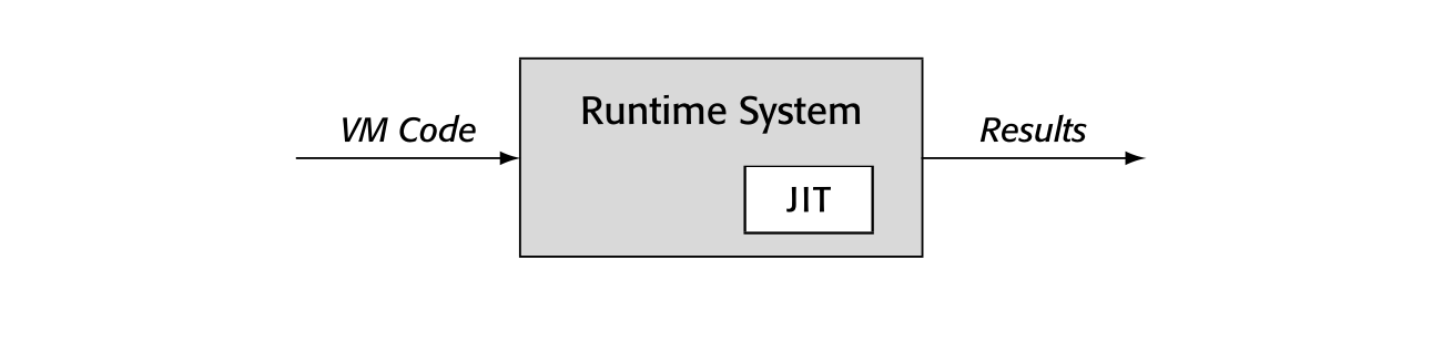
In the classic execution model for compiled code, the processor reads operations and data directly from the address space of the running process. The drawing labeled "Normal Execution" in the margin depicts this situation. (It is a simplified version of Fig. 15.) The fetch-decode-execute cycle uses the processor's hardware.

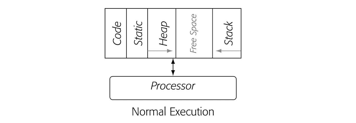
Conceptually, a native-code hot-trace optimizer sits between the executing process' address space and the processor. It "monitors" execution until it has "enough" context to determine that some portion of the code is hot and should be optimized. At that point, it optimizes the code and ensures that future executions of the optimized sequence run the optimized copy rather than the original code. The margin drawing depicts that situation.

The hot-trace optimizer has a difficult task. It must find hot traces. It must improve those traces enough to overcome the costs of finding and compiling them. For each cycle spent in the jit, it must recover one or more cycles through optimization. In addition, if the process slows execution of the cold code, the optimized compiled code must also make up that deficit.

This section presents the design of a hot-trace optimizer. The design follows that of the Dynamo system built at Hewlett-Packard Research around the year 2000. It serves as both an introduction to the issues that arise and a concrete example to explore design tradeoffs.

Dynamo executed native code by emulation until it identified a hot trace. The emulator ran all of the cold code, gathered profile information, and identified the hot traces. Thus, emulated execution of the native code was slower than simply running that code on the hardware. The premise behind Dynamo was that improvement from optimizing hot traces could make up for both the emulation overhead and the jit compilation costs.

These design concepts raise several critical issues. How should the system define a trace? How can it find the traces? How does it decide a trace is hot? Where do optimized traces live? How does emulated cold code link to the hot code and vice versa?

14.3.1 Trace-Entry Blocks

In Dynamo, trace profiling, trace identification, and linking hot and cold code all depend on the notion of a trace-entry block. Each trace starts with an entry block. A trace-entry block meets one of two simple criteria. Either it is the target of a backward branch or jump, or it is the target of an exit from an existing compiled trace.

The first criterion selects blocks that are likely to be loop-header blocks. These blocks can be identified with an address comparison; if the target address is numerically smaller than the current program counter (PC), the target address designates a trace-entry block.

The second criterion selects blocks that may represent alternate paths through a loop. Any side exit from a trace becomes a trace-entry block. The jit identifies these blocks as it compiles a hot trace.

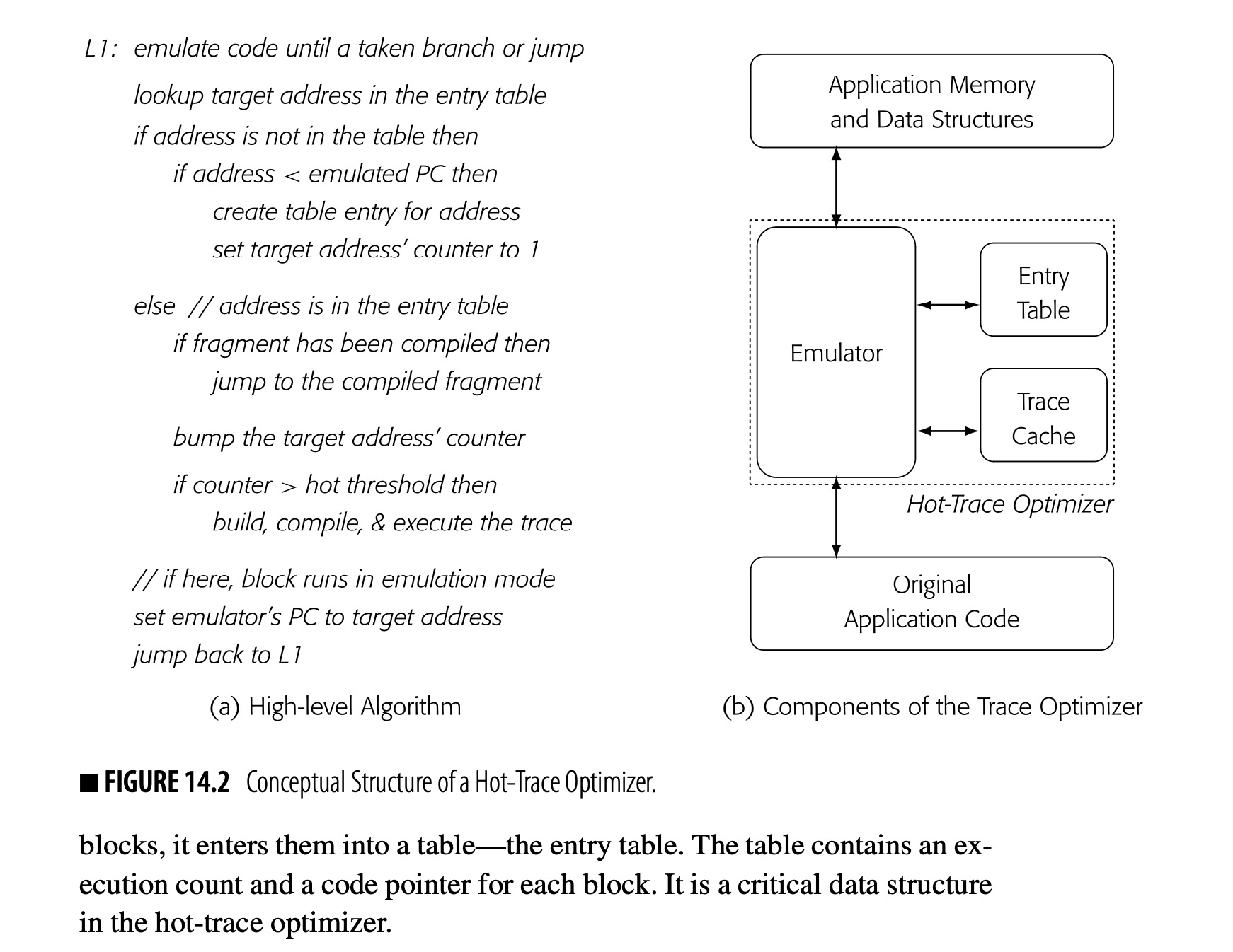
To identify and profile traces, the trace optimizer finds trace-entry blocks and counts the number of times that they execute. Limiting the number of profiled blocks helps keep overhead low. As the optimizer discovers entry blocks, it enters them into a table--the entry table. The table contains an execution count and a code pointer for each block. It is a critical data structure in the hot-trace optimizer.

14.3.1 Flow of Execution

Fig. 14.2(a) presents a high-level algorithm for the trace optimizer. The combination of the trace-entry table and the trace cache encapsulates the system's current state. The algorithm determines how to execute a block based on the presence or absence of that block in the entry table and the values of its execution counter and its code pointer.

Blocks run in emulation until they become part of a compiled hot trace. At that point, further executions of the compiled trace run the block as part of the optimized code. If control enters the block from another off-trace path, the block executes in emulation using the original code.

The critical set of decisions occurs when the emulator encounters a taken branch or a jump. (A jump is always taken.) At that point, the emulator looks for the target address in the trace entry table.

The smaller target address means that this branch or jump is a backward branch.

If the target address is not in the table and that address is numerically smaller than the current PC, the system classifies the target address as a trace entry block. It creates an entry in the table and initializes the entry’s execution counter to one. It then sets the emulator’s PC to the target address and continues emulation with the target block.
If, instead, the target address already has a table entry and that entry has a valid code pointer, the emulator transfers control to the compiled code fragment. Depending on the emulator’s implementation, discussed below, this transfer may require some brief setup code, similar to the precall sequence in a classic procedure linkage.

The compiled trace is stored in the trace cache.

Each exit path from the compiled trace either links to another compiled trace or ends with a short stub that sets the emulator’s PC to the address of the next block and jumps directly back to the emulator—to label $L 1$ in Fig. 14.2(a).

Section 14.3.2 discusses how the compiler can link compiled traces together.

If the target address is in the table but has not yet been compiled, the system increments the target address' execution counter and tests it against the hot threshold. If the counter is less than or equal to the threshold, the system executes the target block by emulation. When the target address' execution counter crosses the threshold, the system builds an IR image of the hot trace, executes and compiles that trace, stores the code into the trace cache, and stores its code pointer into the appropriate slot in the trace entry table. On exit from the compiled trace, execution continues with the next block. Either the code links directly to another compiled trace or it uses a path-specific exit stub to start emulation with the next block.

The algorithm in Fig. 14.2(a) shows the block-by-block emulation, interspersed with execution of optimized traces. The emulator jumps into optimized code; optimized traces exit with code that sets the emulator's PC and jumps back to the emulator. The rest of this section explores the details in more depth.

Emulation

Values that live in memory can use the same locations in both execution modes.

Following Dynamo, the trace optimizer executes cold code by emulation. The JIT-writer could implement the emulator as a full-fledged interpreter with a software fetch-decode-execute loop. That approach would require a simulated set of registers and code to transfer register values between simulated registers and physical registers on the transitions between emulated and compiled code. This transitional code might resemble parts of a standard linkage sequence.

As an alternative, the system could "emulate" execution by running the original compiled code for the block and trapping execution on a taken branch or jump. If hardware support for that trap is not available, the system can store the original operation and replace it with an illegal instruction--a trick used in debuggers since the 1960s.

When the PC reaches the end of the block, the illegal instruction traps. The trap handler then follows the algorithm from Fig. 14.2(a), using the stored operation to determine the target address. In this approach, individual blocks execute from native code, which may be faster than a software fetch-decode-execute loop.

Building the Trace

When a trace-entry block counter exceeds the hot threshold, the system invokes the optimizer with the address of the entry block. The optimizer must then build a copy of the trace, optimize that copy, and enter the optimized fragment into the trace cache.

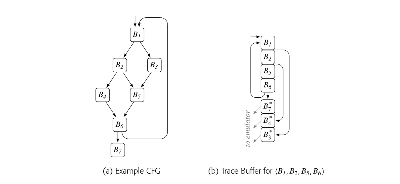
While the system knows that the entry block has run more than threshold times, it does not actually know which path or paths those executions took. Dynamo assumes that the current execution will follow the hot path. Thus, the optimizer starts with the entry block and executes the code in emulation until it reaches the end of the trace--a taken backward branch or a transfer to the entry of a compiled trace. Again, comparisons of runtime addresses identify these conditions.

As the optimizer executes the code, it copies each block into a buffer. At each taken branch or jump, it checks for the trace-ending conditions. An untaken branch denotes a side exit from the trace, so the optimizer records the target address so that it can link the side exit to the appropriate trace or exit stub. When it reaches the end of the trace, the optimizer has both executed the trace and built a linearized version of the code for the JIT to optimize.

Consider the example shown in Fig. 14.3(a). When the emulator sees $B_{I}$ 's counter cross the hot-threshold, it invokes the optimizer. The optimizer executes $B_{I}$ and copies each of its operations into the buffer. The next branch takes control to $B_{2}$ ; the emulator executes $B_{2}$ and adds it to the buffer. Next, control goes to $B_{5}$ followed by $B_{6}$ . The branch at the end of $B_{6}$ goes back to $B_{I}$ , terminating the trace. At this point, the buffer contains $B_{I}$ , $B_{2}$ , $B_{5}$ , and $B_{6}$ , as shown in panel (b).

The drawing assumes that each of the side exits leads to cold code. Thus, the JIT builds a stub to handle each side exit and the end-of-trace exit. The stub labeled $B_{i}^{*}$ sets the emulator's pc to the start of block $B_{i}$ and jumps to the emulator. The stub also provides a location where the optimizer can insert any code needed to interface the compiled code with the emulated code. Panel (b) shows stubs for $B_{3}$ , $B_{4}$ , and $B_{7}$ .

The optimizer builds the trace based on the dynamic behavior of the executing code, which can produce complex effects. For example, a trace can extend through a procedure call and, with a simple callee, through a return. Because call and return are implemented with jumps rather than branches, they will not trigger the criteria for an exit block.

extend through a procedure call and, with a simple callee, through a return. Because call and return are implemented with jumps rather than branches, they will not trigger the criteria for an exit block.

Optimizing the Trace

Once the optimizer has constructed a copy of the trace, it makes one or more passes over the trace to analyze and optimize the code. If the initial pass is a backward pass, the optimizer can collect Live information and other useful facts. From an optimization perspective, the trace resembles a single path through an extended basic block (see Section 8.5). In the example trace, an operation in $B_{6}$ can rely on facts derived from any of its predecessors, as they all must execute before control can reach this copy of $B_{6}$ .

The mere act of trace construction should lead to some improvements in the code. The compiler can eliminate any on-trace jumps. For each early exit, the optimizer should make the on-trace path be the fall-through path. This linearization of the code should provide a minor performance improvement by eliminating some branch and jump latencies and by improving instruction-cache locality.

The compiler writer must choose the optimizations that the JIT will apply to the trace. Value numbering is an obvious choice; it eliminates redundancies, folds constants, and simplifies algebraic identities.

If the trace ends with a branch to its entry block, the optimizer can unroll this path through the loop. In a loop with control flow, the result may be a loop that is unrolled along some paths and not along others--a situation that does not arise in a traditional AOT optimizer.

Early exits from the trace introduce complications. The same compensation-code issues that arise in regional scheduling apply to code motion across early exits (e.g., at the ends of $B_{I}$ and $B_{2}$ ). If optimization moves an operation across an exit, it may need to insert code into the stub for that exit.

Partially dead An operation is partially dead at point $p$ in the code if it is live on some paths that start at $p$ and dead on others.

The optimizer can detect some instances of dead or partially dead code. Consider an operation that defines $r_{i}$ . If $r_{i}$ is redefined before its next on-trace use, then the original definition can be moved into the stubs for any early exits between the original definition and the redefinition. If it is not redefined but not used in the trace, it can be moved into the stubs for the early exits and into the final block of the trace.

After optimization, the compiler should schedule operations and perform register allocation. Again, the local versions of these transformations can be applied, with compensation code at early exits.

Trace-Cache Size

The size of the trace cache can affect performance. Size affects multiple aspects of trace-cache behavior, from memory locality to the costs of lookups and managing replacements. If the cache is too small, the jtt may discard fragments that are still hot, leading to lost performance and subsequent re-compilations. If the cache is too large, it may retain code that has gone cold, hurting locality and raising lookup costs. Undoubtedly, compiler writers need to tune the trace-cache size to the specific system characteristics.

14.3.2 Linking Traces

One key to efficient execution is to recognize when other paths through the cfg become hot and to optimize them in a way that works well with the fragments already in the cache.

In the ongoing example, block $B_{I}$ became hot and the optimizer built a fragment for $⟨ B_{I}, B_{2}, B_{5}, B_{6} ⟩$ , as shown in Fig. 14.4(a). The early exits to $B_{3}$ and $B_{4}$ then make those blocks into trace-entry blocks. If $B_{3}$ becomes hot, the optimizer will build a trace for it. The only trace it can build is $⟨ B_{3}, B_{5}, B_{6} ⟩$ , as shown in panel (b).

If the optimizer maintains a small amount of information about trace entries and exits, it can link the two traces in panel (b) to create the code shown in panel (c). It can rewrite the branch to $B_{1}^{*}$ as a direct jump to $B_{1}$ . Similarly, it can rewrite the branch to $B_{3}^{*}$ as a direct jump to $B_{3}$ . The interlinked traces then create fast execution paths for both $⟨ B_{I}, B_{2}, B_{5}, B_{6} ⟩$ and $⟨ B_{I}, B_{3}, B_{5}, B_{6} ⟩$ , as shown in panel (c). The exits to $B_{4}$ and $B_{7}$ still run though their respective stubs to the interpreter. 1

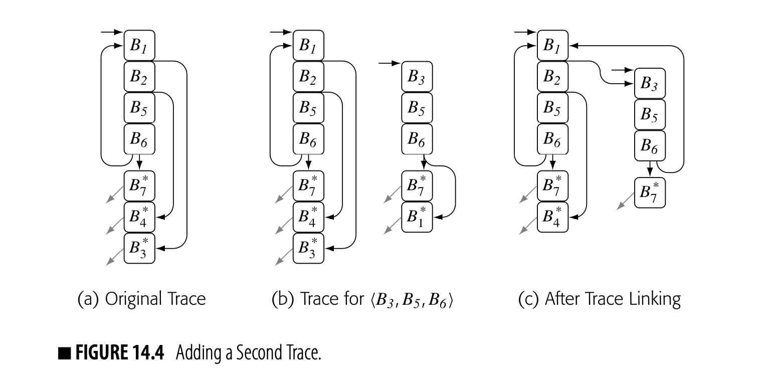
If during optimization of $⟨ B_{I}, B_{2}, B_{5}, B_{6} ⟩$ , the JIT moved operations into $B_{3}^{*}$ , then the process of linking would need to either (1) preserve $B_{3}^{*}$ on the path from $B_{I}$ to $B_{3}$ or (2) prove that the operations in $B_{3}^{*}$ are dead. With a small amount of context, such as the set of registers defined before use in the fragment, it could recognize dead compensation code in the stub.

Cross-linking in this way also addresses a weakness in the trace-construction heuristic. The trace builder assumed that the $(k + 1)$ st execution of $B_{I}$ took the hot path. Because the system only instruments trace header blocks, $B_{I}$ 's execution count could have accrued from multiple paths between $B_{I}$ and $B_{6}$ . What happens if the $(k + 1)$ st execution takes the least hot of those paths?

With trace linking, the $(k + 1)$ st execution will build an optimized fragment. If that execution does not follow the hot path, then one or more of the early exits in the fragment will become hot; the optimizer will compile them and link them into the trace, capturing the hot path or paths. The optimizer will recover gracefully as it builds a linked set of traces.

Intermediate Entries to a Trace

In the example, when $B_{I}$ became hot, the system built an optimized trace for $⟨ B_{I}, B_{2}, B_{5}, B_{6} ⟩$ . When $B_{3}$ became hot, it optimized $⟨ B_{3}, B_{5}, B_{6} ⟩$ .

The algorithm, as explained, builds a single trace for $⟨ B_{I}, B_{2}, B_{5}, B_{6} ⟩$ and ignores the intermediate entry to the trace from the edge $(B_{3}, B_{5})$ . The system then executes the path $⟨ B_{3}, B_{5}, B_{6} ⟩$ by emulation until $B_{3}$ 's counter triggers compilation of that path. This sequence of actions produces two copies of the code for $B_{5}$ and $B_{6}$ , along with the extra JIT-time to optimize them.

Another way to handle the edge $(B_{3}, B_{5})$ would be to construct an intermediate entry into the trace $⟨ B_{I}, B_{2}, B_{5}, B_{6} ⟩$ . The trace-building algorithm, as explained, ignores these intermediate entry points, which simplifiesrecord-keeping. If the emulator knew that $B_{5}$ was an intermediate entry point, it could split the trace on entry $B_{5}$ . It would build an optimized trace for $⟨ B_{1}, B_{2} ⟩$ and another for $⟨ B_{5}, B_{6} ⟩$ . It would link the expected-case exit from $⟨ B_{1}, B_{2} ⟩$ to the head of $⟨ B_{5}, B_{6} ⟩$ .

$B_{4}$ has one predecessor while $B_{5}$ has two.

To implement trace splitting, the optimizer needs an efficient and effective mechanism to recognize an intermediate trace entry point--to distinguish, in the example, between $B_{4}$ and $B_{5}$ . The hot-trace optimizer, as described, does not build an explicit representation of the CFG. One option might be for the AOT compiler to annotate the VM code with this information.

Splitting $⟨ B_{1}, B_{2}, B_{5}, B_{6} ⟩$ after $B_{2}$ may produce less efficient code than compiling the unsplit trace. Splitting the trace avoids compiling $⟨ B_{5}, B_{6} ⟩$ a second time and storing the extra code in the code cache. It requires an extra slot in the entry block table. This tradeoff appears to be unavoidable. The best answer might well depend on the length of the common suffix of the two paths, which may be difficult to discern when compiling the first trace.

Selection Review

A hot-trace optimizer identifies frequently executed traces in the running code, optimizes them, and redirects future execution to the newly optimized code. It assumes that frequent execution in the past predicts frequent execution in the future and focuses the JIT's effort on such "hot" code. The acyclic nature of the traces leads to the use of local and superlocal optimizations. Those methods are fast and can capture many of the available opportunities.

The use of linked traces and interprocedural traces lets a hot-trace optimizer achieve a kind of partial optimization that an ahead-of-time compiler would not. The intent is to focus the JIT's effort where it should have maximum effect, and to limit its effort in regions where the expected impact is small.

Review Questions

Once a trace entry block becomes hot, the optimizer chooses the rest of the trace based on the entry-block's next execution. Contrast this strategy with the trace-discovery algorithm used in trace-scheduling. How might the results of these two approaches differ?
Suppose the trace optimizer fills its trace cache and must evict some trace. What steps would be needed to revert a specific trace so that it executes by VM-code emulation?

14.4 Hot-Method Optimization

Method-level optimization presents a different set of challenges and trade-offs than does trace-level optimization. To explore these issues, we will first consider a hot-method optimizer embedded in a JAVA environment. Our design is inspired by the original HotSpot Server Compiler (hereafter, HotSpot). The design is a mixed-mode environment that runs cold methods as JAVA bytecode and hot methods as native code. We finish this section with a discussion of the differences in a native-code hot-method optimizer.

14.4.1 Hot-Methods in a Mixed-Mode Environment

Fig. 14.5 shows an abstract view of the JAVA virtual machine or JVM. Classes and their associated methods are loaded into the environment by the Class Loader. Once stored in the VM, methods execute on an emulator--the figure's "Bytecode Engine." The JVM operates in a mixed-mode environment, with native-code implementations for many of the standard methods in system libraries.

To add a method-level JIT, the compiler writer must add several features to the JVM: the JIT itself, a software-managed cache for native-code method bodies, and appropriate interfaces. Fig. 14.6 shows these modifications.

From an execution standpoint, the presence of a JIT brings several changes. Cold code still executes via VM-code emulation; methods from native libraries still execute from native code. When the system decides that a method is hot, it JIT-compiles the VM code into native code and stores the 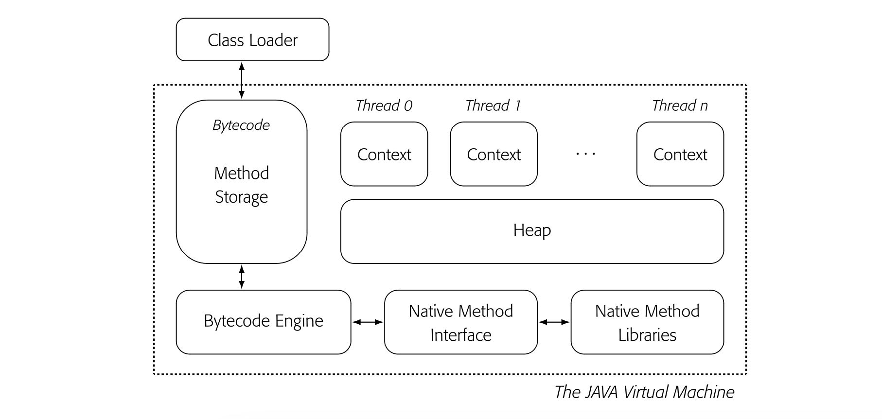new code in its native-code cache. Subsequent calls to that method run from the native code, unless the system decides to revert the method to VM-code emulation (see the discussion of deoptimization on page 742).

Using native-code ARs may necessitate translation between native-code and VM- code formats.

The JAVA community often refers to ARs as “stack frames.”

The compiler writer must make several key decisions. The system needs a mechanism to decide which methods it will compile. The system needs a strategy to gather profile information efficiently. The compiler writer must decide whether the native code operates on the VM-code or the native-code versions of the various runtime structures, such as activation records. The compiler writer must design and implement the JIT, which is just an efficient and constrained compiler. Finally, the compiler writer must design and implement a mechanism to revert a method to VM-code emulation when the compiled method proves unsuitable. We will explore these issues in order.

Trigger for Compilation

Conceptually, the hot-method optimizer should compile a method when that method consumes a significant fraction of the execution time. Finding a hot method that meets this criterion is harder than finding a hot trace, because the notion of a "significant fraction" of execution time is both imprecise and unknowable until the program terminates.

Iteration can occur with either loops or recursion. The mechanism should catch either case.

Thus, hot-method optimizers fall back on counters and thresholds to estimate a method's activity. This approach relies on the implicit assumption that a method that has consumed significant runtime will continue to consume significant runtime in the future. Our design, following HotSpot, will measure: (1) the number of times the method is called and (2) the number of times of loop iterations that it executes. Neither metric perfectly captures the notion that a method uses a large fraction of the running time. However, any method that does consume a significant fraction of runtime will almost certainly have a large value in one of those two metrics.

THE HOTSPOT SERVER COMPILER

Around 2000, Sun Microsystems delivered a pair of JITs for its JAVA environment: one intended for client-side execution and the other for server-side execution. The original HotSpot Server Compiler employed more expensive and extensive techniques than did the client-side JIT. The HotSpot Server compiler was notable in that it used strong global optimization techniques and fit them into the time and space constraints of a JIT. The authors used an IR that explicitly represented both control flow and data flow [92]. The IR, in turn, facilitated redundancy elimination, constant propagation, and code motion. Sparsity in the IR helped make these optimizations fast.

The JIT employed a novel global scheduling algorithm and a full coloring allocator (see Section 13.4). To make the coloring allocator practical, the authors developed a method to trim the interference graph that significantly shrank the graph. The result was a state-of-the-art JIT that employed algorithms once thought to be too expensive for use in a JIT.

The system can “sum” the counters by using a single location for all the counters in a method.

Thus, the system should count both calls to a method and loop iterations within a method. Strategically placed profile counters can capture each of these conditions. For call counts, the system can insert a profile counter into each method's prolog code. For iteration counts, the system can insert a profile counter before each loop-closing branch. To trigger compilation, it can either use separate thresholds for loops and invocations, or it can sum the counters and use a single threshold.

HotSpot counted both calls and iterations and triggered a compilation when the combined count exceeded a preset threshold of 10,000 events. This threshold is much larger than the one used in Dynamo (50). It reflects the more aggressive and expensive compilation in HotSpot.

Runtime Profile Data

To capture profile data, compiler writers can instrument either the VM code for the application or the implementation of the VM-code engine.

Instrumented VM Code. The system can insert VM code into the method to increment and test the profile counters. In this design, the profile overhead executes as VM code. Either the AOT compiler or the Class Loader can insert the instrumentation. Counter for calls can be placed in the method's prolog code, while counters for a specific call-site can be placed in the appropriate precall sequence.

To profile loop iterations, the transformation can insert a counter into any block that is the target of a backward branch or jump. An AOT strategy might decrease the cost of instrumentation; for example, if the AOT compiler knows the number of iterations, it can increment the profile counter once for the entire loop.

Instrumented Engine. The compiler writer can embed the profile support directly into the implementtaion of the VM-code engine. In this scheme, the emulator's code for branches, jumps, and the call operation (e.g., the JVM's invokestatic or invokevirtual) can directly increment and test the appropriate counters, which are stored at preplanned locations. Because the profile code executes as native code, it should be faster than instrumenting the VM code.

By contrast, an AOT compiler would find loop headers using dominators (see Sec- tion 9.2.1).

The emulator could adopt the address comparison strategy of the trace optimizer to identify loop header blocks. If the target address is numerically smaller than the PC, the targeted block is a potential loop header. Alternatively, it could rely on the AOT compiler to provide an annotation that identifies loop-header blocks.

Compiling the Hot Method

Tree-pattern matching techniques are a good match to the constraints of a JIT (see Section 11.4).

When profile data triggers the JIT to compile some method $x$ , the JIT can simply retrieve the VM code for $x$ and compile it. The JIT resembles a full-fledged compiler. It parses the VM code into an IR, applies one or more passes of optimization to the IR, and generates native code--performing instruction selection, scheduling, and register allocation. The JIT writes that native code into the native-code cache (see Fig. 14.6). Finally, it updates the tables or pointers that the system uses to invoke methods so that subsequent calls map to the cached native code.

In a mixed-mode environment, the benefits of JIT compilation should be greater than they are in a native-code environment because the cold code executes more slowly. Thus, a hot-method optimizer in a mixed-mode environment can afford to spend more time per method on optimization and code generation. Hot-method optimizers have applied many of the classic scalar optimizations, such as value numbering, constant propagation, dead-code elimination, and code motion (see Chapters 8 and 10). Compiler writers choose specific techniques for the combination of compile-time efficiency and effectiveness at improving code.

Global value numbering

The literature on method-level JITs often mentions global value numbering as one of the key optimizations that these JITs employ. The dutiful student will find no consensus on the meaning of that term. Global value numbering has been used to refer to a variety of distinct and different algorithms.

One approach extends the ideas from local value numbering to a global scope, following the path taken in superlocal and dominator-based value numbering (DVNT). These algorithms are more expensive than DVNT and the cost-benefit tradeoff between DVNT and the global algorithm is not clear.

Another approach uses Hopcroft's partitioning algorithm to find operations that compute the same value, and then rewrites the code to reflect those facts. The HotSpot Server compiler used this idea, which fit well with its program dependence graph IR.

Finally, the JIT writer could work from the ideas in lazy code motion (LCM). This approach would combine code motion and redundancy elimination. Because LCM implementations solve multiple data-flow analysis problems, the JIT writer would need to pay close attention to the cost of analysis.

Optimizations

Hot-method JITs apply local, regional, and global optimizations. Because the JIT operates at runtime, the compiler writer can arrange for an optimization to access the runtime state of the executing program to obtain runtime values and use them in optimization.

Value Numbering Method-level JITs typically apply some form of value numbering. It might be a regional algorithm, such as DVNT, or it might be one of a number of distinct global algorithms.

Value numbering is attractive to the JIT writer because these techniques achieve multiple effects at a relatively low cost. Typically, these algorithms perform some subset of redundancy elimination, code motion, constant propagation, and algebraic simplification.

Inline method caches can provide site- specific data about receiver types. The idea can be extended to capture type information on parameters, as well.

Specialization to Runtime Data A JIT can have access to data about the code's behavior in the current execution, particularly values of variables, type information, and profile data. Runtime type information lets the JIT speculate; given that a value consistently had type $t$ in the past, the JIT assumes that it will have type $t$ in the future.

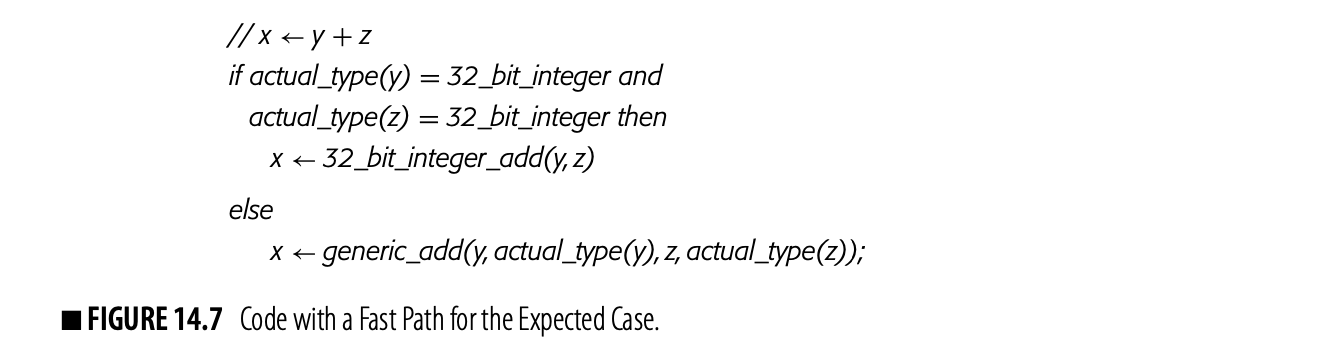
Such speculation can take the form of a fast-path/slow-path implementation. Fig. 14.7 shows, conceptually, how such a scheme might work. The code assumes that $x$ and $y$ are both 32-bit integers and tests for that case;if the test fails, it invokes the generic addition routine. If the slow path executes too many times, the system might recompile the code with new speculated types (see the discussion of "deoptimization" on page 742).

Inline Substitution The JIT can inline calls, which lets it eliminate method lookup overhead and call overhead. Inlining leads the JIT to tailor the callee's body to the environment at the call site. The JIT can use data from inline method caches to specialize code based on call-site specific type data. It can also inline call sites in the callee; it should have access to profile data and method cache data for all of those calls.

When a JIT considers inline substitution, it has access to all of the code for the applica- tion. In an AOT compiler, that situation is unlikely.

The JIT can also look back to callers to assess the benefits of inlining a method into one or more of its callers. Again, profile data on the caller and type information from the inline cache may help the JIT make good decisions on when to inline.

Code Generation Instruction selection, scheduling, and register allocation can each further improve the JIT-compiled code. Effective instruction selection makes good use of the ISA's features, such as address modes. Instruction scheduling takes advantage of instruction-level parallelism and avoids hardware stalls and interlocks. Register allocation tries to minimize expensive spill operations.

The challenge for the JIT writer is to implement these passes efficiently. Tree-pattern matching techniques for selection combine locally optimal code choice with extreme JIT-time efficiency. Both the scheduler and the allocator can capitalize on sparsity to make global algorithms efficient enough for JIT implementation. The HotSpot Server Compiler demonstrated that efficient implementations can make these global techniques not only acceptable but advantageous.

As with any JAVA system, a JIT should also try to eliminate null-pointer checks, or move them to places where they execute less frequently. Escape analysis can discover objects whose lifetimes are guaranteed to be contained within the lifetime of some method. Such objects can be allocated in the method's AR rather than on the heap, with a corresponding decrease in allocation and collection costs. Final and static methods can be inlined.

Deoptimization

Deoptimization the JIT generates less optimized code due to changes in runtime information

If the JIT uses runtime information to optimize the code, it runs the risk that changes in that data may render the compiled code either badly optimized or invalid. The JIT writer must plan for reasonable behavior in the event of a failed type speculation. The system may decide to deoptimize the code.

To “notice,” the system would need to in- strument the slow path.

Consider Fig. 14.7 again. If the system noticed, at some point, that most executions of this operator executed the generic_odd path, it might recompile the code to speculate on another type, to speculate on multiple types, or to not speculate at all. If the change in behavior is due to a phase-shift in program behavior, reoptimization may help.

If, however, the statement has simply stopped showing consistency in the types of $x, y$ , or $z$ , then repeated reoptimization may be the wrong answer. Unless the compiled code executes enough to cover the cost of JIT compilation, the recompilations will slow down execution.

The alternative is to deoptimize the code. Depending on the precise situation and the depth of knowledge that the JIT has about temporal type locality, it might use one of several strategies.

If the JIT knows that the actual type is one of a small number, it could generate fast path code for each of those types.
If the JIT knows nothing except that the speculated type is often wrong, it might generate unoptimized native code that just calls generic_odd or it might inline generic_odd at the operation.
If the JIT has been called too often on this code due to changing patterns, it might mark the code as not fit for JIT compilation, forcing the code to execute in emulation.

A deoptimization strategy allows the JIT to speculate, but limits the downside risk of incorrect speculation.

14.4.2 Hot-Methods in a Native-Code Environment

Several issues change when the JIT writer attempts hot-method optimization in a native-code environment. This section builds on insights from the Deutsch-Schiffman SMALLtalk-80 implementation.

Initial Compilations

The native-code environment must ensure that each method is compiled to native code before it runs. Many schemes will work, including a straightforward AOT compilation, load-time compilation of all methods, or JIT compilation on the first invocation, which we will refer to as compile oncall. The first two options are easier to implement than the last one. Neither, however, creates the opportunity to use runtime information during that initial compilation.

Using an indirect pointer to the code body (a pointer to a pointer) may simplify the implementation.

A compile-on-call system will first generate code for the program's main routine. At each call site, it inserts a stub that (1) locates the VM code for the method; (2) invokes the JIT to produce native code for the method; and (3) relinks the call site to point to the newly compiled native code. When the execution first calls method $m$ , it incurs a delay for the JIT to compile $m$ and then executes the native-code version of $m$ . If runtime facts are known, the first call to $m$ can capitalize on them.

If the JIT compiler supports multiple levels of optimization, the compiler writer must choose which level to use in these initial compiles. A lower level of optimization should reduce the cost of the initial JIT compiles, at the cost of slower execution. A higher level of optimization might increase the cost of the initial JIT compiles, with the potential benefit of faster execution.

To manage this tradeoff, the system may use a low optimization level in the initial compiles and recompile methods with a higher level of optimization when they become hot. This approach, of course, requires data about execution frequencies and type locality.

Gathering Profile Data

In a native-code environment, the system can gather profile information in two ways: instrument the code to collect profile data at specific points in the code, or shift to interrupt-driven techniques that discover where the executable spends its time.

Instrumented Code. The JIT compiler can instrument code as described earlier for a mixed-mode hot-method optimizer. The JIT can insert code into method prologs to count total calls to the method. It can obtain call-site specific counts by adding code to precall sequences. It can insert code to count loop iterations before loop-closing branches.

With instrumented code, JIT invocation proceeds in the same way that it would in the mixed-mode environment. The JIT is invoked when execution counts, typically call counts and loop iterations, pass some preset threshold. For a loop-iteration count, the code to test the threshold and trigger compilation should be inserted, as well.

To capture opportunities for type speculation and type-based code specialization, the JIT can arrange to record the type or class of specific values--typically, parameters passed to the method or values involved at a call in the method. The JIT should have access to that information.

Interrupt-Driven Profiles Method-invocation counts tell the system how often a method is called. Iteration counts tell the system how often a loop body executes. Neither metric provides insight into what fraction of total running time the instrumented code actually uses.

The system must produce tables to map an address into a specific location in the original code.

A native-code environment spends virtually all of its time executing application code. Thus, it can apply another strategy to discover hot code: interrupt-driven profiling. In this approach, the system periodically stops execution with a timer-driven interrupt. It maps the program-counter address at the time of the interrupt back to a specific method, and increments that method's counter. Comparing the method's counter against the total number of interrupts provides an approximation to the fraction of execution time spent in that method.

Some systems have used a combination of instrumented code and interrupt-driven profile data.

Because an interrupt-driven profile measures something subtly different than instrumented code measures, the JIT writer should expect that an interrupt-driven scheme will optimize different methods than an instrumented code scheme would.

The JIT still needs data, when possible, on runtime types to guide optimization. While some such data might exist in inline method caches at call sites, the system can only generate detailed information if the compiler adds type-profiling code to the executable.

Deoptimization with Native Code

When a compiled method begins execution, it must determine if the preconditions under which it was compiled (e.g., type or class speculation, constant valued parameters, etc.) still hold. The prolog code for a method can test any preconditions that the JIT assumed in its most recent compilation. In a mixed-mode environment, the system could execute the VM code if the precondition check fails; in a native-code environment, it must invoke the JIT to recompile the code in a way that allows execution to proceed.

In a recompilation, the system should attempt to provide efficient execution while avoiding situations where frequent recompilations negate the benefits of JIT compilation. Any one of several deoptimization strategies might make sense.

This strategy suggests a counter that limits the number of “phase shifts” the JIT will tolerate on a given method.

The JIT could simply recompile the code with the current best runtime information. If the change in preconditions was caused by a phase shift in program behavior, the current preconditions might hold for some time.
If the JIT supports multiple levels of optimization--especially with regard to type speculation--the system could instruct the JIT to use a lower level of speculation, which would produce more generic and lesstailored code. This approach tries to avoid the situation where the code for some method oscillates between two or more optimization states.
An aggressive JIT could compile a new version of the code with the current preconditions and insert a stub to choose among the variant code bodies based on preconditions. This approach trades increased code size for the possibility of better performance.

The best strategy will depend on how aggressively the JIT uses runtime information to justify optimizations and on the economics of JIT compilation. If the JIT takes a small fraction of execution time, the JIT writer and the user may be more tolerant of repeated compilations. By contrast, if it takes multiple invocations of a method to compensate for the cost of JIT compilation, then repeated recompilations may be much less attractive than lowering the level of speculation and optimization.

The Economics of JIT Compilation

The fundamental tradeoff for the JIT writer is the difference between cycles spent in the JIT and cycles saved by the JIT. In a native-code environment, the marginal improvement from the JIT may be lower, simply because the unoptimized code runs more quickly than it would in a similar mixed-mode environment.

This observation, in turn, should drive some of the decisions about which optimizations to implement and how much recompilation to tolerate. The JIT writer must balance costs, benefits, and policies to create a system that, on balance, improves runtime performance.

Section Review

A hot-method optimizer finds procedures that either execute frequently or occupy a significant fraction of execution time. It optimizes each procedure in light of the runtime facts that it can discern. Because a method optimizer can encounter control flow, it can benefit from regional and global optimizations, such as global value numbering or code motion; these transformations have higher costs and, potentially, higher payoffs than the local and superlocal techniques available to a trace optimizer.

The tradeoffs involved in a specific design depend on the execution environment, the source-language features that produce inefficiency, and the kinds of information gathered in the runtime environment. The design of a hot-method optimizer requires an understanding of the language, the system, the algorithms, and the behavior of the targeted applications.

14.5 Advanced Topics

The previous sections introduce the major issues that arise in the design of a runtime optimizer. To build such a system, however, the compiler writer must make myriad design decisions, most of which have an impact on the effectiveness of the system. This section explores several major topics that arise in the literature that surrounds jit compilation. Each of them has a practical impact on system design. Each of them can change the overall efficacy of the system.

14.5.1 Levels of Optimization

In practice, we know few developers who consider compile time when selecting an optimization level.

AOT compilers typically offer the end user a choice among multiple levels of optimization. This feature allows the user, in theory, to use stronger optimization in places where it matters, while saving on compile time in places where the additional optimization makes little difference.

A jit-based system might provide multiple levels of optimization for several reasons.

Because the elapsed time for application execution includes the jit's execution, the jit writer may decide to include in the standard compilation only those optimizations that routinely produce improvements.
The system may find that a native-code fragment executes often enough to justify more extensive analysis and optimization, which requires more jit time and saves more runtime.
If the jit performs speculation based on runtime information, such as types and classes, the jit may later need to deoptimize the code, which suggests a lower level of optimization.

For all these reasons, some runtime optimization systems have implemented multiple levels of optimization.

If the system discovers a loop with a large iteration count, it might apply loop-specific optimizations, such as unrolling, strength reduction, or code motion. To ensure that those changes have immediate effect, it could perform on-stack replacement (see Section 14.5.2).

If the system finds that one method accounts for a significant fraction of interrupt-based profile points, it might apply deeper analysis and more intense optimization. For example, it might inline calls, perform analyses to disambiguate types and classes, and reoptimize.

In either of these scenarios, a JIT with multiple levels of optimization needs a clear set of policies to govern when and where it uses each level of optimization. One key part of that strategy will be a mechanism to prevent the JIT from trying to change the optimization level too often--driving up the JIT costs without executing the code enough to amortize the costs.

14.5.2 On-Stack Replacement

A method-level JIT can encounter a situation in which one of the profile counters crosses its threshold during an execution of a long-running method. For example, consider a method with a triply nested loop that has iteration counts of 100 at each level. With a threshold of 10,000, the counter on the inner loop would trigger compilation after just one percent of the iterations.

In effect, the system behaves as if a long- running method has a higher threshold to trigger compilation.

The counter shows that the method is hot and should be optimized. If the system waits until the next call to "install" the optimized code, it will run the current code for the rest the current invocation. In the triply nested loop, the code would run 99 percent of the iterations after the counter had crossed the threshold for optimization.

To avoid this missed opportunity, the system could pause the execution, optimize and compile the code, and resume the execution with the improved code. This approach capitalizes on the speed of the compiled code for the majority of the loop iterations. To resume execution with the newly optimized code, however, the system must map the runtime state of the paused execution into the runtime state needed by the newly optimized code.

On-stack code replacement A technique where the runtime system pauses execution, JIT compiles the execut- ing procedure, and resumes execution with the newly compiled code

This approach, optimizing the procedure in a way that the current invocation can continue to execute, is often called on-stack code replacement. The JIT builds code that can, to the extent possible, execute in the current runtime environment. When it cannot preserve the values, it must arrange to map values from the current environment into the new environment.

The JIT can use its detailed knowledge of the old code to create the new environment. It can generate a small stub to transform the current environment--values in registers plus the current activation record--into the environment need by the new code.

The stub may need to move some values. The storage map of the new code may not match the storage map of the old code.
The stub may need to compute some values. Optimizations such as code motion or operator strength reduction may create new values that did not exist in the original code.
The stub may be able to discard some values. The state of the original code may contain values that are dead or unused in the new code.

The stub runs once, before the first execution of the new code. At that point, it can be discarded. If the jit runs in a separate thread, as many do, the system needs some handshaking between the jit and the running code to determine when it should switch to the new code.

The compiler writer has several ways to reduce the complexity of on-stack replacement.

She can limit the number of points in the code where the system can perform replacement. The start of a loop iteration is a natural location to consider. Execution of the next iteration begins after compilation and state mapping.

Techniques that create compensation code or introduce new values can complicate the mapping. Examples include code motion, software pipelining, and inline substitution.

She can simplify the state-mapping problem by limiting the set of optimizations that the jit uses when compiling for on-stack replacement. In particular, the jit might avoid techniques that require significant work to map the old environment into the new one.

The implementation of on-stack replacement ties in a fundamental way to the interfaces between emulated and compiled codes and their runtime environments. The details will vary from system to system. This strategy has the potential to provide significant improvement in the performance of long-running methods.

14.5.3 Code Cache Management

To avoid confusion, we will refer to the JIT’s cache as a $co d e c a c h e$ and to processor caches as hardware caches.

Almost all jit-based systems build and maintain a code cache--a dedicated, software-managed block of memory that holds jit-compiled code. The jit writer must design policies and build mechanisms to manage the code cache. Conceptually, code caches blend the problems and policies of a hardware cache and a software-managed heap.

Hardware caches determine an object's placement by an arithmetic mapping of virtual addresses to physical addresses. In a heap, software searches for a block of free space that will hold the object. Code caches are closer to the heap model for placement.
Hardware caches deal with fixed sized blocks. Heaps deal with requests for arbitrarily sized blocks, but often round those requests to some common sizes. Code caches must accommodate blocks of native code of different sizes.
Hardware caches use automatic, policy-based eviction schemes, typically informed by the pattern of prior use. Heaps typically run a collection phase to find blocks that are no longer live (see Section 6.6.2). Code caches use policies and mechanisms similar to hardware caches.

Most JIT-based systems have a separate code cache for each process or each thread. Some JIT writers have experimented with a global code cache, to allow the reuse of JIT compiled code across processes. The primary benefit from these designs appears to be a reduction in overall memory use; they may provide better performance for a multitasked environment on a limited memory system. When these systems find cross-process sharing, they also avoid reinvoking the JIT on previously compiled code, which can reduce overall runtimes.

If virtual memory is fast enough, the system can make the cache large and let the paging algorithms manage the problem.

The use of a limited-size code cache suggests that the standard virtual-memory paging mechanism is either too slow or too coarse-grained to provide efficient support for the JIT-compiled code. Use of a limited-size cache also implies that a code-cache eviction will discard the JIT-compiled code; delimiting it from the executing program and necessitating either emulation or a recompilation if it is invoked in the future.

Replacement Algorithm

When the JIT compiles code, it must write that code into the code cache. If the cache management software cannot find a block of unused memory large enough to hold the code, it must evict another segment from the cache.

A direct-mapped hardware cache has a set size of one.

Replacement in the code cache differs from replacement in a hardware cache. A set-associative hardware cache determines the set to which the new block maps and evicts one of the set's blocks. The literature suggests evicting the least recently used (Lru) block; many hardware caches use or approximate Lru replacement.

Code cache management algorithms need to evict enough segments to create room for the newly compiled code. In a hardware cache, eviction involves a single fixed-size line. In a software-managed code cache, allocation occurs at the granularity of the segment of compiled code (a trace, a method, or multiple methods). This complicates both the policy and the implementation of the replacement algorithm.

The cache management software should evict from the code cache one or more segments that have not been used recently. The evicted segmentsmust free enough space to accommodate the new code without wasting "too much" space. Choosing the LRU segment might be a good start, but the potential need to evict multiple segments complicates that decision. If the new code requires eviction of multiple segments, those segments must be adjacent. Thus, implementing an LRU mechanism requires some additional work.

The final constraint on replacement is that the algorithms must be fast; any time spent in the replacement algorithms adds to the application's running time. Creative engineering is needed to minimize the cost of choosing a block to evict and of maintaining the data structures to support that decision.

Fragmentation

Repeated allocation and replacement can fragment the space in a code cache. Collected heaps address fragmentation with compaction; uncollected heaps try to merge adjacent free blocks. Code caches lack the notion of a free command; in general, it is unknowable whether some code fragment will execute in the future, or when it will execute.

If the system executes in a virtual-memory environment, it can avoid some of the complication of managing fragmentation by using more virtual address space than allocated memory. As long as the code cache's working set remains within the intended cache size, the penalty for using more virtual address space should be minimal.

14.5.4 Managing Changes to the Source Code

This feature is not new. Both APL in the 1960s and Smalltalk in the 1970s had fea- tures to edit source code. Those systems, however, were built on interpreters.

Some languages and systems allow runtime changes to an application at the source-code level. Interpreted environments handle these changes relatively easily. If the runtime environment includes JIT-compiled code, the system needs a mechanism to recognize when a change invalidates one or more native-code fragments, and to replace or recompile them.

The runtime system needs three mechanisms. It must recognize when change occurs. It must identify the code and data that the change affects. Finally, it must bring the current runtime state into agreement with the new source code.

Recognize Change

The system must know when the underlying code has changed. The most common way to capture changes is by restricting the mechanisms for making a change. For example, JAVA code changes require the class loader; in APL, code changes involved use of the quote-quad operator. The interface that allows the change can alert the system.

Identify Scope of Change

Similar problems arise with interprocedu- ral optimization in an AOT compiler (see Section 8.7.3).

The system must understand where the changes occur. If the text of a procedure fee changes, then native code for fee is undoubtedly invalid. The system needs a map from a procedure name to its native-code implementation. The more subtle issues arise when a change in fee affects other procedures or methods.

If, for example, the jit previously inlined fee into its caller foe, then the change to fee also invalidates the prior compilation of foe. If fee is a good target for inline substitution--say, its code size is smaller than the standard linkage code--then a change to fee might trigger a cascade of recompilations. The map from procedure names to code bodies becomes multivalued.

Interface changes to a method, such as changing the parameters, must invalidate both the changed procedure and all of the procedures that call it. Details in the precall and postreturn sequences are inferred from the interface; if it changes, those sequences likely change, too.

Recompiling Changed Code

At a minimum, the system must ensure that future calls to a method execute the most recent code. In a mixed-mode environment, it may suffice to delete the jit-compiled code for a changed method and revert to interpreting the vm code. When the method becomes hot again, the system will compile it. In a native-code environment, the system must arrange for the new code to be compiled--either aggressively or at its next call.

To simplify recompilation, the jit writer might add a level of indirection to each call. The precall sequence then refers to a fixed location for the callee; the jit stores a pointer to the code body at that location. The extra indirection avoids the need to find all of the callers and update their code pointers. To relink the method, the jit simply overwrites the one code pointer.

In the case where the changed code invalidates compilations of other procedures, the number of invalidations can rise, but the same basic mechanisms should work.

Changes to Dedarations

Runtime changes to the source code introduce a related problem--one that arises in both interpreted and compiled implementations. If the source code can change, then the definitions of data objects can change. Consider, for example, a change that adds a new data member to a class. If that class already has instantiated objects, those objects will lack the new data member. The source language must define how to handle this situation, but in theworst case, the system might need to find and reformat all of the instantiated instances of the class--a potentially expensive proposition.

To simplify finding all of the objects in a class, the system might link them together. Early smalltalk systems exhaustively searched memory to find such objects; the limited memory on those systems made that approach feasible.

14.6 Summary and Perspective

Just-in-time compilation systems make optimization and code generation decisions at runtime. This approach can provide the jit compiler with access to more precise information about names, values, and bindings. That knowledge, in turn, can help the jit specialize the code to the actual runtime environment.

jit systems operate under strict time constraints. Well-designed and well-built systems can provide consistent improvements. The speedups from the jit must compensate for the time spent gathering information, making decisions, and compiling code. Thus, jit writers need a broad perspective on language implementation and a deep knowledge of compilation and optimization techniques.

Despite the long history of runtime optimization, the field remains in flux. For example, one of the most heavily used jit, Google's v8 JavaScriptJIT, was originally written as a native-code, compile-on-call system. Experience led to a reimplementation that uses a mixed-mode, hot-method approach. The primary justification for this change given in the literature was to reduce code space and startup time; the hot-method version also avoided parsing unused code. Changes in languages, runtime environments, and experience have driven work in runtime optimization over the last decade. We anticipate that this field will continue to change for years to come.

Chapter Notes

Runtime compilation has a long history. McCarthy included a runtime compilation facility in his early LISP system so that it could provide efficient execution of code that was constructed at runtime--a direct consequence of LISP's unified approach to code and data [266].

Thompson used an "edit-time" compilation of regular expressions into naive code for the IBM 7094 to create a powerful textual search tool for his port of the QED editor [345]; Section 2.4.2 describes the underlying construction.

Hansen built his Adaptive Fortran system to explore the practicality and profitability of runtime optimization [188]. It supported a subset of fortran iv and a small set of optimizations. He modeled the behavior of his system against widely known fortran compilers of the time. His dissertation includes significant discussion on how to estimate the benefits of an optimization and how to trigger the runtime optimizations.

The Deutsch-Schiffman Smalltalk-80 implementation, built for an early Sun Microsystems workstation, demonstrated the potential of runtime compilation for improving dynamic languages [137]; contemporary implementations that relied on interpreting Smalltalk bytecode ran more slowly.

The HotSpot Server Compiler [288] and Dynamo [32] were widely recognized and influential systems. HotSpot influenced design decisions in jit-based systems for a decade or more. Dynamo inspired a generation of work on problems that ranged from code-cache management to software dynamic translation.

Most method-level optimizers apply some form of global value numbering. These algorithms range from global extensions of the ideas in local value numbering [59, 167] through algorithms that build on Hopcroft's dfa minimization algorithm [90, 312] to implementations of lazy code motion (see the notes for Chapter 10).

The time constraints that arise in jit compilation have encouraged the use of efficient algorithms. Tree-pattern matching instruction selectors can be hyper-efficient: using five to ten compile-time operations per emitted operation [162, 163, 297]. Linear scan register allocation avoids the expensive part of a full-fledged coloring allocator: building the interference graph [296]. In an environment where many methods are small and do not require spill code, linear scan works well. The HotSpot Server Compiler used interference graph trimming to reduce the cost of a full-fledged coloring allocator [93].

Exercises

Consider again the plot in Fig. 10 (Java scaling with and without the jit). How might changes in the threshold for jit compilation affect the behavior of the jit-enabled curve, particularly at the lower end of the curve, shown in panel (b)?
Write pseudocode for a backward pass over an acyclic trace that discovers dead and partially dead operations. Assume that the jit has live information at each exit from the trace. How might the jit obtain live information for the trace exits?* One consideration in the design of a hot-trace optimizer is how to handle intermediate entries into a trace. The design in Section 14.3 ignores intermediate entries, with the effect that multiple copies of some blocks are made. As an alternative, the compiler writer could have the trace-building algorithm split the trace at an intermediate entry. This strategy would generate an optimized trace for the portion before the intermediate entry and an optimized trace for the portion after the intermediate entry. It would then directly link the former part to the latter part.

How might the trace-building algorithm recognize that a block is an intermediate entry point?
What kinds of JIT optimizations might have reduced effectiveness as a result of splitting traces around intermediate entry points?
If the trace optimizer has a bounded code cache and it fills that cache, it may need to evict one or more traces.
What complications do linked traces introduce?
What approaches can the code-cache management algorithms take to managing the eviction of linked traces?
When a system with a hot-method optimizer discovers that some method has triggered too many recompilations, it may decide to de-optimize the method. The JIT could treat individual call sites differently, linking each call site to an appropriately optimized code body for the method.
What information should the system gather to enable such call-site specific optimization and deoptimization?
What additional runtime data structures might the JIT need in order to implement such call-site specific optimization?
One obvious cost of such a scheme is space in the code cache. How might the compiler writer limit the proliferation of variant code bodies for a single method?
Some hot-method JIT compile code in a separate thread, asynchronously. What advantages might this offer to the end user? What disadvantages might it create?
Deoptimization must deal with the results of inline substitution. Suppose the JIT has inlined fie into fee, and that it later decides that it must deoptimize fee. What strategies can the JIT implement to simplify deoptimization of a method that includes inlined code?* 8. Ahead-of-time (AOT) compilers choose which procedures to inline based on some combination of static analysis and profile data from a prior run on "representative" data. By contrast, a JIT decides to inline a procedure based almost entirely on runtime profile information. 1. Suggest three heuristics that a hot-method JIT might use to determine whether or not to inline the callee at a specific call site. 2. What kinds of data can the runtime system gather to help in the decision of whether or not to inline a specific call site? 3. Contrast your strategies, and the results you expect from them, with the results you expect from an AOT compiler.